Machine Learning for Hydraulic Francis Runner Design Optimization

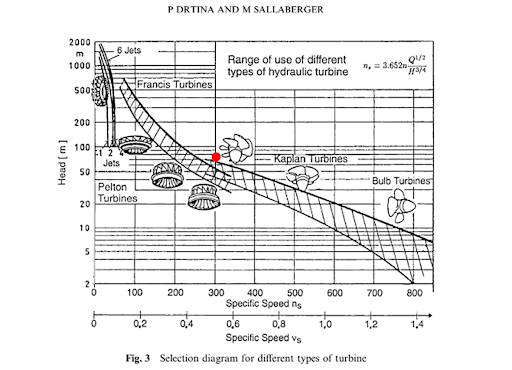
Electricity generation through hydropower is a key option in the portfolio of clean, renewable energy, and at the heart of many of these systems lies the Francis runner. This mixed flow rotor is the most widely used type of hydraulic turbine today, being extremely versatile, making it the ideal choice for sites with a medium head (the vertical distance the water falls, typically from 30 to 600 meters) and a very wide range flow rates from less than 1, to 100s of cubic metres per second. Its widespread adoption is a testament to the broader advantages of hydropower itself: a reliable energy source that provides grid stability that now plays a crucial role in the global transition to sustainable carbon-free power.

However, a large share of the current installed hydropower was built many years ago, before the appearance of modern digital tools. The average age of the existing hydropower installations in Europe is 46 years and 50 years in the United States. So the turbomachinery itself will not be optimised for fully efficient performance across a range of operating conditions. There is an opportunity then to re-evaluate what it means to have an efficient Francis runner design that can fully deliver all the advantages of hydropower.

In this blog we look at how ADT’s Reactive Response Surface + CAE technology (RRS+CAE) is driving better hydraulic turbine design through Machine Learning. 

• The Francis Runner performance challenge - and the solution
• Where to start - Generate a meanline Francis runner design
• 3D Inverse Design is the enabling technology for Machine Learning
• How to establish a baseline for turbine performance
• Optimization of a Francis runner via Machine Learning
• RRS gives design choices and performance gains
• Final validation of the Machine Learning solution
• Conclusions

The challenge is to create a new generation of Francis runners which (a) deliver exceptional performance and (b) work efficiently across a range of power and flows as the grid demand and the natural variations in reservoir head change the operating conditions whilst remaining, crucially, at a constant rotor speed.

TURBOdesign Suite from Advanced Design Technology (ADT) brings Machine Learning methods to the realm of Francis runner design to create stages that are optimised for multiple objectives across multiple operating points. Let’s take a look at how a highly efficient and optimised design can be arrived at in just a few hours when we let the Machine Learning system take the reins.

Where to start - Generate a meanline Francis runner design

Before the ML system can get to grips with optimizing a Francis runner design, we need to establish a baseline sizing and component integration for the stage, based on the most basic requirements of the hydraulic turbine:

TD-Pre creates the Francis turbine stage geometry from a set of minimum requirements, to which we could also add specific constraints such as vane and runner maximum diameters, if we were, for example, re-rating existing hydropower plant.

Plugging these numbers into TURBOdesign Pre, plus some other details about the working fluid, the inlet conditions, and how the stage should be configured results in a complete 2D stage design for the runner and all the associated components if required (volute, stay vanes and guide vanes).

 

Fig1: TURBOdesign-Pre results for inverse meanline design calculation of a Francis turbine design specification

This inverse approach (define operating point - obtain the geometry as a result) is far more efficient and much quicker than attempting to design the entire stage by ‘trying out’ many and various geometries and then discovering what the performance might be - the so called ‘direct design’ approach. Even if that discovery process is using low-fidelity models rather than full-fidelity 3D CFD to simulate performance, the ‘misses’ (designs that do not satisfy the basic performance requirements) are going to vastly outnumber the ‘hits’ (designs that meet the specs).

So, by using inverse design we instantly have a realisable complete stage design that would meet the requirements of the basic duty specified. It may not be the most efficient, or have performance at other operating points, but these extended performance requirements will come from the Machine Learning process which we’ll set up.

 

Fig 2: Complete Francis turbine stage design realized in CAD: Volute, stay vanes, guide vanes and runner

3D Inverse Design is the enabling technology for Machine Learning

In a previous blog, we showed how ADT have constructed and assembled the necessary building blocks to enable a turbomachinery Machine Learning system that can rapidly and efficiently home in on optimized designs. In that case the application was an axial fan, but as you’d expect, the system can be configured to work on any turbomachinery design challenge. Very briefly, the advantages of 3D Inverse Design over conventional design are:

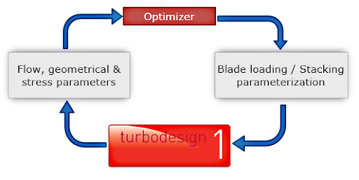
Coupled with ADT’s Reactive Response Surface (RRS) optimizer technology, vast and complex turbomachinery design spaces can be explored and exploited in a matter of hours on standard desktop hardware.

How to establishing a baseline for turbine performance

We can import our meanline design directly into TURBOdesign1 (TD1) which will create the 3D blade shape based on the distribution of blade loading and the required duty. A baseline design can use the default loading distribution provided and this will take the design most of the way. Then we can drive an optimum design based upon more specific,  mutli-objective and multi-point performance objectives.

We now set up a CFD simulation to discover the performance at multiple operating points. For this study we are going to fix the onset angle of the flow to 60° - which simulates a fixed upstream guide vane angle, and vary the flow rate between 410 and 500 kg/s, simulating a low, design, and high power demand from the grid.  TD1 integrates seamlessly with major CFD systems including ANSYS-CFX and Simcentre Star CCM+ . So just a couple of mouse-clicks have the CFD runs underway. Domain creation, meshing, pre-processing, running the solver and post-processing are templated, scripted processes, managed by TD1, so we get consistency of analysis time after time.

 

Fig 3: TURBOdesign1 seamlessly integrates with high-fidelity simulation to create performance data for multiple operating points

Once the CFD is completed we have our baseline characteristic for efficiency versus flow and required head versus power for a fixed rotor speed of 1350 rpm.

 

Fig4: Baseline characteristics for efficiency, flow, head and power

Now let's see how much improvement in performance we can get.

Optimization of a Francis runner via Machine Learning

Inputs

The power of 3D Inverse Design means that we can use just 10 input parameters to create a large and rich design space wherein we hope to find a significantly better performing optimal design. 4 of the parameters relate the distribution of blade loading across the blade, 4 control the meridional shape, 1 governs the trailing edge wrap angle or ‘chevron’ and the final parameter is blade number. So we have a combination of continuous and discrete variables in the design space. Navigating this hybrid space is a serious challenge for many optimizers, however the Reactive Response Surface algorithm is attuned to this possibility as blade number is such an obvious and crucial driver of rotor performance. We are greatly aided here by the small number of continuous variables needed - if we had many hundreds of input variables, as typically used in a direct design optimization (blade angles and stacking at multiple points along multiple streamlines) then the combinatorial explosion would fatally hinder the optimization search.

TD1 also uses an Machine Learning algorithm to recommend appropriate ranges for your input variables, so that the design space is not too wide, resulting in ‘impossible’ designs, nor too narrow which might preclude a genuine, usable optimum being found. This pre-conditioning boosts the ‘hit-rate’ during the design space exploration, avoiding combinations of input parameters that cannot be solved in the inverse design problem.

 

Fig5: The entire blade design space is described in just 10 parameters

Constraints

We apply a constraint to the optimizer algorithm - limiting the blade maximum lean to no more than 40 degrees. This to ensure a reasonable mechanical design that can be manufactured. During the optimization process RRS+CAE recognizes constraint violations and knows to move the search away from areas which are producing invalid designs.

Objectives

What do we want from this machine? Here is the real power of the Reactive Response Surface+CAE method - because we are integrating multi-point CFD runs into this study we can choose CFD results as objectives. So we do not need to know about the intricacies of the 3D flow field or how it interacts with the rotor. We can simply ask for increased efficiency at each operating point and to maximise the value of Pmin, that is, the minimum pressure on the blade. We do not care how the Machine Learning algorithm solves this task - we only care about the outcome. With 4 objectives (efficiency at each of 3 operating points, plus Pmin), we will have a 4-dimensional solution space.

Once we have set the optimizer meta-parameters (number of iterations, number of new designs added per iteration, and some settings governing the surrogate model used within RRS + CAE) the optimizer can be run to find the optimum solution.

RRS gives design choices and performance gains

Reactive Response Surface + CAE uses a combination of low- and high fidelity simulation, surrogate models and a genetic algorithm to discover the optimum designs. In this case we discover a Pareto front of candidate designs in 4 dimensions (1 dimension for each of the objectives). Every point on this front - as shown below - is an optimal compromise between the 4 objectives.  So we can select a final design based on what priorities we choose - effectively weighting the objectives based on relative importance. At this stage, these are all surrogate model points, so have not been ‘realized’ as actual blade shapes and assessed in higher-fidelity simulation.

In this case we can choose 2 options: the peak efficiency performing design, which happens to have 14 blades (the baseline has 13) , and the design which maximises Pmin (so has the greatest cavitation margin) which has 16 blades.

 

Fig 6: Surrogate Pareto front of optimal solutions - minimum pressure vs stage efficiency. All points on this plot are Pareto optimal, we are viewing a 4-dimensional front in 2 dimensions. The chosen optima are highlighted.

For any surrogate model point we can run the candidate through 3D Inverse Design to generate the actual blade shape, and then send to CFD under the same meshing, pre-processing and boundary conditions as the baseline and optimization points to get a final assessment of performance.  By doing so we find that both our chosen optima return a very good improvement over the baseline in all objectives:

 

Fig7: Optimized characteristics (red, orange) show significant improvement over the baseline (blue)

We have significantly improved impeller efficiency (5-9 points) at all conditions. We have also increased shaft power for the same head by an astonishing 8-28% with a large increase in cavitation margin.

 

Fig8: Surface minimum pressure (abs kPa)The design optimized for increased minimum pressure on the blade delivers significantly increased cavitation margin

 

Fig9: Baseline Francis Runner geometry (left) compared with optimized (for Peak Pmin) geometry (right) 

Final validation of the Machine Learning solution

It is very important to assess how accurate the design space surrogate model is. We must have confidence in the Reactive Response Surface model to correctly predict the shape of the design space, otherwise we would be adding in high-fidelity simulation to predict multi-point performance at the ‘wrong’ Pareto front. The comparison between the Reactive Response Surface surrogate model prediction and verification in CFD for the peak efficiency optimum design is shown below.

 

We find that the actual CFD performance results agree extremely well with the predicted surrogate Reactive Response Surface values to within a maximum error of less than 0.2% on the objectives and the predicted power, showing that Reactive Response Surface + CAE is an extremely accurate method for predicting the design space topology.

We can also validate the inverse design approach by checking the actual distribution in the CFD prediction of the key inverse design parameter rVΘ* . This is the spanwise distribution of work and should match between what the inverse design specifies as an input, and how the blade actually performs when run in CFD.

 

Fig10: Top left shows the input spanwise distribution of work for TURBOdesign1, the 3 other plots show the actual distributions of the same in CFD

The four plot figure above makes the important point that, viscous effects notwithstanding, all the blade designs perform to the required duty specified as an input by the inverse design tool. This is why inverse design is so effective for optimization: whilst you can explore a large, variant design space, including changes in blade number, the key performance parameters for every candidate in the design space remain close to the original requirements.

Conclusions

In this blog we have shown that, in just a few hours on a standard workstation, Reactive Response Surface + CAE can discover significant Francis runner performance gains with component redesign using the 3D Inverse Design approach. Moreover that design can be validated with high confidence in full-fidelity CFD to confirm what the Reactive Response Surface surrogate model predicts.

The Reactive Response Surface + CAE model is an ideal method for delivering optimal designs in a multi-point, multi-objective design space, and for a fraction of the total cost traditionally associated with large scale, high-fidelity optimisation studies involving complex geometry and flow interaction.