Machine Learning for Centrifugal Pump Design

TL;DR

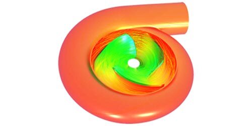
The design of efficient centrifugal pumps is being revolutionized by combining 3D Inverse Design with a Reactive Response Surface (RRS) Machine Learning optimizer. Using only 5 input parameters, this methodology efficiently explores a multi-objective design space and took just 5 hours to generate an optimized impeller. The resulting pump design successfully achieved goals like increased Net Positive Suction Head (NPSH) to prevent cavitation and higher overall efficiency across various flow rates, all while maintaining strict constraints on power and head rise.

Here are some eye-opening numbers that should make you think about the design of efficient pumps
●    More than 20% of the world's electricity supply is used to power liquid pumps
●    Rotodynamic pumps account for 80% of the installed base
●    Pumps are the largest industrial consumer of electricity across Europe. Requiring 300 TW.hours per year, which drives over 65 million tons of CO₂ emissions.

So even small improvements in efficiency and performance scale up into huge gains, both economically and ecologically.

In this blog we look at how ADT’s Rapid Response Surface + CAE technology is driving better pump design through Machine Learning.

●    The centrifugal pump performance challenge - and the solution
●    The starting point for centrifugal pumps - creating a meanline design
●    3D Inverse Design - the enabling technology for Machine Learning
●    Establishing baseline pump performance 
●    Turbomachinery design optimization via Machine Learning 
●    Centrifugal pump design choices and optimized performance gains
●    Validation of pump design performance confirms Machine Learning solution 
●    Conclusions - Machine Learning for turbomachinery design is now a reality

The centrifugal pump performance challenge - and the solution

The challenge is to create a new generation of centrifugal pumps which (a) deliver exceptional baseline performance and (b) work efficiently across a range of speeds and flows as dictated by the mass introduction of variable speed drives over the last decade.

TURBOdesign Suite from Advanced Design Technology (ADT) brings Machine Learning methods to the field of centrifugal pump design to create stages that are optimised for multiple objectives across multiple operating points. Let’s take a look at how a highly efficient and optimised design can be arrived at in just a few hours when we let the Machine Learning system take the reins.

The starting point for centrifugal pumps - creating a meanline design

Before the ML system can get to grips with optimizing a design, we need to establish a baseline sizing and component integration for the stage, based on the most basic requirements of the pump:
●    How much flow
●    How much head (pressure rise)
●    How fast will it spin

Plugging these numbers into TURBOdesign Pre, plus some other details about the working fluid, the inlet conditions, and how the stage should be configured results in a complete 2D stage design for the centrifugal pump rotor and all the associated components if required (diffuser, impeller, volute, return channel).

 

Figure 1: TD-Pre creates the meanline design of the pump stage, calculated from the duty requirements

Within seconds we also get an approximation of the characteristics across the speed and flow range. Using this starting point, we know that we are on the right track for a well-conditioned, correctly sized machine.

 

Figure 2: TD-Pre also generates the characteristic performance curves for the design

3D Inverse Design - the enabling technology for Machine Learning

In a previous blog, we showed how ADT have constructed and assembled the necessary building blocks to enable a turbomachinery Machine Learning system that can rapidly and efficiently home in on optimized designs.

In that case the application was an axial fan, but as you’d expect, the system can be configured to work on any turbomachinery design challenge.

Very briefly, the advantages of 3D Inverse Design over conventional design are:
●    Minimization of input parameters. Just a handful of parameters are required to describe extremely complex and varied 3D blade shapes.
●    Parameter leverage. Small changes to parameter values can drive large blade shape changes.
●    Designs are guaranteed to meet duty points. As the required performance is the input and the blade shape is the output, 3D Inverse Design does not waste effort creating non-compliant designs that do not meet the basic performance requirements. 
●    Designs can be assessed for performance without reverting to high-fidelity, and high-cost CFD simulation.

Coupled with ADT’s Reactive Response Surface (RRS) optimizer technology, vast and complex turbomachinery design spaces can be explored and exploited in a matter of hours on standard deskside hardware.

Establishing baseline pump performance
 We can import our centrifugal pump meanline design directly into TURBOdesign1, which will create the 3D blade shape based on the distribution of blade loading and the required duty. A baseline design can use the default loading distribution provided and this will take the design most of the way. Then we can drive an optimum design based upon more specific,  multi-objective and multi-point performance objectives.

One click to start the 3D Inverse design solver and 30 seconds later we have our baseline centrifugal pump design along with detailed estimations of centrifugal pump performance at the design point. 

We now set up a CFD simulation to discover the centrifugal pump performance at the off-design points. For this study, we’ll look at 85% and 115% flowrates. To do this TURBOdesign1 integrates seamlessly with major CFD systems including ANSYS-CFX , Simcenter STAR-CCM+ and Cadence Fine Turbo

So just a couple of mouse-clicks have the CFD runs underway. Domain creation, meshing, pre-processing, running the solver and post-processing are templated, scripted processes, managed by TURBOdesign1, so we get consistency of analysis time after time. 

Once the CFD is completed we have our baseline centrifugal pump characteristic for efficiency and head versus flow along this speedline. 

 

Figure 3: Baseline characteristics for efficiency and head

Now let's see how much improvement in performance we can get.

 Turbomachinery design optimization via Machine Learning 

Inputs

The power of 3D Inverse Design means that we can use just 5 input parameters to create a large and rich design space wherein we hope to find a significantly better performing optimal design. 4 of the parameters relate the distribution of blade loading across the blade, and the 5th controls the width of the trailing edge. TURBOdesign1 also uses an Machine Learning algorithm to recommend appropriate ranges for your input variables, so that the design space is not too wide, resulting in ‘impossible’ designs, nor too narrow which might preclude a genuine, usable optimum being found. This innovation, combined with a smart understanding of constraints (see below) means the the Reactive Response Surface Machine Learning method requires many fewer datapoints than other gradient or genetic based optimizers.  Accelerating the time to survey the design space in the search for the optimum centrifugal pump design.

 

 Figure 4: The entire blade design space is described in just 5 parameters

Constraints

All good optimization algorithms work with constraints in order to efficiently explore design space. Reactive Response Surface + CAE recognizes constraint violations and knows to move the search away from these areas. In this case we constrain the throat area to limit the flow rate change. We also constrain the power and head rise, which will drive us toward more efficient centrifugal pump designs, not just more powerful ones.

Objectives

What outcomes do we want from this centrifugal pump design ? Because we are integrating multi-point CFD runs into this study we can choose CFD results from off-design points as objectives. In words, we want to increase the pump's Net Positive Suction Head (NPSH) to avoid cavitation, and increase the overall efficiency. So in TURBOdesign1 we tell the Reactive Response Surface optimizer to maximize Pmin and maximize OP2 (low flow) efficiency and OP3 (high flow) efficiency. Note that because head rise and power are constrained, the optimizer cannot solve this problem just by making the pump consume more power and generate more head, it must come up with an efficient design answer within the constraints.

Once we have set the optimizer meta-parameters (number of iterations, number of new designs added per iteration, and some settings governing the surrogate model used within Reactive Response Surface + CAE) the optimizer can be run to find the optimum solution.

Because the Reactive Response Surface + CAE makes very selective use of high-fidelity CFD to explore the multi-objective, multi-point design space, this optimization took just 5 hours on 11 cores of a deskside Xeon workstation.

Centrifugal pump design choices and optimized performance gains

The Reactive Response Surface + CAE method uses a combination of low- and high-fidelity simulation, surrogate models and a genetic algorithm to discover the optimum centrifugal pump designs.

In this case, we discover a Pareto front of candidate centrifugal pump designs in 3 dimensions (1 dimension for each of the objectives). Every point on this front - as shown below - is an optimal compromise between the 3 objectives.  

So we can select a final design based on what priorities we choose - effectively weighting the objectives based on relative importance. At this stage, these are all surrogate model points, so have not been ‘realized’ as actual blade shapes and assessed in higher-fidelity simulation.

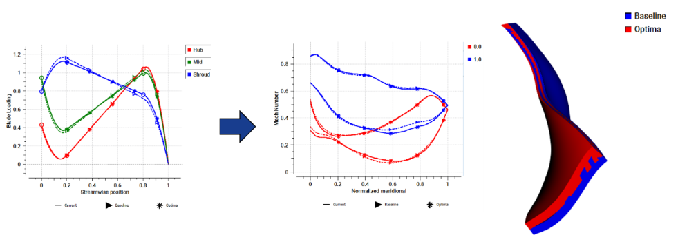
In this case, we choose a centrifugal pump design which pays-off minimum pressure against efficiency at the low flow (OP2) point. Highlighted in the plot below:

 

Figure 5: Surrogate Pareto front of optimal solutions - minimum pressure vs impeller efficiency. All points on this plot are Pareto optimal, we are viewing a 3-dimensional front in 2 dimensions. The chosen optimal is highlighted in blue.

 

Figure 6: Baseline centrifugal pump geometry (left) compared with optimized geometry (right) 

For any surrogate model point we can run the candidate through 3D Inverse Design to generate the actual blade shape, and then send to CFD under the same meshing, pre-processing and boundary conditions as the baseline and optimization points to get a final assessment of performance. By doing so we find that our chosen optimum centrifugal pump returns a very good improvement over the baseline in all objectives:

 

Figure 7: Optimized characteristics (red) show significant improvement over the baseline (blue)

Figure 7 reveals that when CFD analysis is repeated on the compound lean nozzle, the loss peak near the endwalls due to passage vortices is found to be lower but the loss at the midspan has increased due to greater loading in this area compared to radial stacking.

Validation of pump design performance confirms Machine Learning solution

It is very important to assess how accurate the design space surrogate model is. We must have confidence in the Reactive Response Surface model to correctly predict the shape of the design space, otherwise we would be adding in high-fidelity simulation to predict multi-point performance at the ‘wrong’ Pareto front. The comparison between the Reactive Response Surface surrogate model prediction and verification in CFD is shown below.

 

Figure 8: Comparison Chart

We find that the actual CFD performance results agree very well with the predicted Reactive Response Surface values to within a maximum error of around 0.1% on all objectives, showing that Reactive Response Surface + CAE is an extremely accurate method for predicting the design space topology.

Conclusions - Machine Learning for turbomachinery design is now a reality

In this blog we have shown that, in just a few hours on a standard workstation, Reactive Response Surface +CAE can discover significant centrifugal pump performance gains with component redesign using the 3D Inverse Design approach. Moreover that design can be validated with high confidence in full-fidelity CFD to confirm what the Reactive Response Surface surrogate model predicts.

The Reactive Response Surface + CAE model is an ideal method for delivering optimal designs in a multi-point, multi-objective design space, and for a fraction of the total cost traditionally associated with large scale, high-fidelity optimisation studies involving complex geometry and flow interaction.